

Some spreadsheet tasks feel wildly more dramatic than they need to be. You open Google Sheets, stare at a column of numbers, and suddenly act like you are defusing a bomb. The good news is that totaling a column in Google Sheets on a PC or Mac is one of the easiest things you can do once you know the trick. Even better, once you learn it, you can use the same idea for budgets, sales reports, grade books, invoices, mileage logs, inventory sheets, and every other document that quietly begs for math.
If you want the fast answer, it is this: use the SUM function. But if you want to actually understand what you are doing, avoid common mistakes, and learn a couple of smarter shortcuts along the way, this guide will walk you through the process step by step. By the end, you will know how to total a column in Google Sheets, how to total an entire column, how to get a quick total without placing a formula, and how to handle filtered data without your spreadsheet getting sneaky.
Why Totals Matter More Than People Admit
There is something deeply satisfying about a clean total at the bottom of a column. It turns random data into information you can actually use. A list of weekly expenses becomes a monthly spending picture. A column of product sales becomes a revenue snapshot. A set of quiz scores becomes a class average starting point. In other words, a total is not just a number. It is the moment your spreadsheet finally starts telling a story.
Google Sheets makes this process simple on desktop, whether you are using a Windows PC or a Mac. The interface is nearly identical in a browser, so the steps below work the same way in Chrome, Safari, Edge, or Firefox.
How to Total a Column on Google Sheets on PC or Mac: 7 Steps
Step 1: Open your Google Sheet and find the column you want to total
Start by opening the spreadsheet that contains your data. Locate the column with the numbers you want to add. For example, maybe column B contains monthly expenses, column D contains sales, or column F tracks hours worked.
Before you do anything else, make sure the cells actually contain numbers. If some entries are text, extra symbols, or oddly pasted values, your total may be wrong or incomplete. A neat-looking column is great. A mathematically cooperative column is better.
Step 2: Click an empty cell where you want the total to appear
Choose a blank cell for the result. Most people place the total directly below the last number in the column, which keeps the sheet easy to read. So if your values run from B2 through B12, you might click cell B13.
You can also place the total somewhere else, such as the top of a summary section or in another part of the sheet. Google Sheets does not care where the answer lives, as long as the formula points to the correct range.
Step 3: Type an equals sign to begin the formula
In the empty cell, type =. Every formula in Google Sheets starts with an equals sign. Think of it as the spreadsheet’s way of saying, “All right, I’m listening. What do you want me to calculate?”
Once you type the equals sign, Google Sheets knows you are entering a formula rather than regular text. That tiny symbol is the door to a lot of spreadsheet power, and today we are walking through it with snacks and confidence.
Step 4: Enter the SUM function
After the equals sign, type SUM and open a parenthesis. Your formula should now look like this:
=SUM(
The SUM function in Google Sheets is designed to add numbers from one or more cells or ranges. As you type, Google Sheets may suggest the function automatically. You can click the suggestion or keep typing manually. Either method works.
Step 5: Select the cells in the column you want to add
Now highlight the cells you want to total with your mouse. If your numbers are in cells B2 through B12, drag through that range. Google Sheets will insert the range reference into the formula for you, so it becomes:
=SUM(B2:B12)
The colon between B2 and B12 tells Google Sheets to include everything from the starting cell to the ending cell. This is the standard way to total a continuous range in one column.
If you already know the range, you can type it manually instead of dragging. That is often faster when you are comfortable with spreadsheet references.
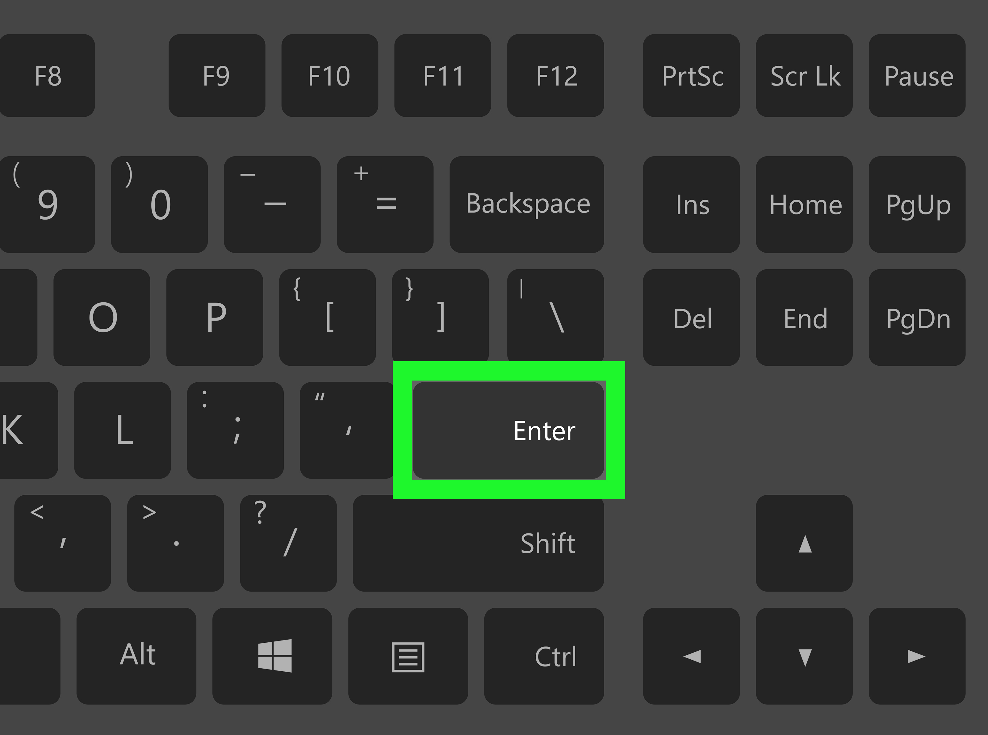
Step 6: Close the parenthesis and press Enter
Type the closing parenthesis if needed, so the full formula is complete:
=SUM(B2:B12)
Then press Enter. Google Sheets will instantly calculate the total and display the result in the selected cell. Congratulations. You have officially told a spreadsheet what to do, and it obeyed. That is a small but meaningful thrill.
Even better, the result updates automatically if the numbers in that range change later. So if B7 changes from 25 to 35, your total changes too. No calculator. No drama. No suspicious napkin math.
Step 7: Adjust the formula when you need a smarter total
The basic total works beautifully for most cases, but a few common variations are worth knowing.
If you want to total an entire column, you can use a formula like this:
=SUM(B:B)
This tells Google Sheets to add everything in column B. It is convenient, especially for columns that keep growing over time. However, it is usually smarter to avoid putting the formula inside the same column you are totaling, or you may create a circular reference and a very grumpy spreadsheet.
If your sheet uses filters or hidden rows and you only want visible values, use SUBTOTAL instead of SUM. For example:
=SUBTOTAL(109,B2:B100)
This version is incredibly useful in reports and dashboards because it ignores hidden rows when appropriate. In plain English, it totals what you can see, not everything lurking in the background like an uninvited spreadsheet ghost.
Example: Totaling a Monthly Budget Column
Let’s say you have a personal budget sheet with expenses in column C:
Rent in C2, groceries in C3, gas in C4, internet in C5, and entertainment in C6. To total those expenses, click C7 and type:
=SUM(C2:C6)
Press Enter, and Google Sheets displays the total monthly spending. If groceries go up because eggs have once again decided they are luxury items, you only change the value in C3. The total updates on its own.
That is the beauty of using formulas instead of typing totals manually. Your spreadsheet becomes dynamic rather than decorative.
How to Get a Quick Total Without Inserting a Formula
Sometimes you do not want to place a formula in the sheet at all. Maybe you just want a quick answer and then want to move on with your day. In that case, highlight the cells you want to add and look at the bottom-right corner of Google Sheets.
You can see summary information there, including a quick Sum. This is handy when you want to check a number fast without modifying the spreadsheet layout. It is basically the spreadsheet equivalent of peeking at the answer key without making a scene.
This quick total is useful for one-off checks, but if you need a number that stays in the document and updates later, use a real formula in a cell.
Common Mistakes When Totaling a Column in Google Sheets
Including the header in the range
If your column has a label such as “Expenses” in B1, do not include that cell unless you want Google Sheets to try to make sense of it. A safer formula is usually =SUM(B2:B12), not =SUM(B1:B12).
Placing the formula inside the range being totaled
If you put your total formula in B12 and also total B2:B12, Google Sheets may run into a circular reference. Translation: the formula is trying to count itself, which is not healthy for spreadsheets or people.
Using text-formatted numbers
If copied values do not sum correctly, they may be stored as text instead of numbers. This happens often when data is pasted from websites, PDFs, or accounting systems. If the total looks suspiciously low, inspect the cells before blaming mathematics as a concept.
Using SUM when you really need SUBTOTAL
If your data is filtered and the total still includes hidden rows, the issue is not that Google Sheets hates you. You are probably using SUM when SUBTOTAL is the better choice.
Useful Variations You Should Know
Total multiple non-adjacent cells
If the cells are scattered, use commas instead of a range:
=SUM(B2,B5,B9)
Total across another sheet tab
If your data lives on a different tab named Sales, you can use:
=SUM(Sales!B2:B20)
Total a growing list
If new values are added regularly, an open-ended range can help:
=SUM(B2:B)
This starts at B2 and keeps going down the column as new rows are added. It is excellent for ongoing trackers, logs, and monthly reports.
Why the SUM Function Is So Beginner-Friendly
Part of what makes Google Sheets approachable is that the SUM formula behaves the way most people expect. You tell it where the numbers are, and it adds them. No weird syntax. No advanced setup. No need to sacrifice a weekend to a spreadsheet course unless you really enjoy that sort of thing.
The function is also flexible. You can total a short range, a full column, multiple separate cells, or even data on another tab. Once you understand the basic pattern, you can scale it up easily.
That is why learning how to total a column in Google Sheets on a PC or Mac is one of the best beginner spreadsheet skills. It is small, practical, and instantly useful.
Real-World Experience: What People Usually Learn After Doing This a Few Times
Here is the funny thing about totaling a column in Google Sheets: the first time you do it, it feels like a tutorial exercise. The fifth time, it feels like a life skill. After you start using Sheets for real projects, you notice that totals show up everywhere. You use them for grocery budgets, side hustle income, freelance invoices, online store orders, workout logs, classroom grades, travel spending, and household bills. Suddenly, the humble SUM function becomes one of the most useful tools on your laptop.
One common experience is realizing that the formula itself is not the hard part. The real challenge is keeping the data clean. People often discover that one odd pasted value, one header accidentally included in the range, or one number stored as text can throw off the total. That moment teaches an important spreadsheet lesson: formulas are only as reliable as the data you feed them. In other words, spreadsheets are honest, but they are not mind readers.
Another experience people have is moving from quick totals to smarter totals. At first, they just want to add a column. Then they start filtering the sheet by month, category, or customer and wonder why the total is not changing the way they expected. That is usually when they meet SUBTOTAL and realize there is a difference between totaling all data and totaling only visible data. It feels like a small discovery, but it can dramatically improve reports and dashboards.
Many users also learn that placement matters. Putting the total directly under the column works well for simple sheets, but in larger files, it often makes more sense to create a summary area. That way, the raw data stays separate from the key metrics. Once people start organizing totals into a summary box, their spreadsheets begin looking less like digital junk drawers and more like actual tools.
There is also the confidence factor. A lot of beginners feel nervous around formulas because they assume spreadsheets are for accountants, analysts, or mysterious people who say things like “pivot that dataset” before breakfast. But totaling a column is often the first formula that makes everything click. Once users see that =SUM(B2:B12) works and updates automatically, they stop being afraid of formulas. Then they try averages, percentages, conditional sums, and eventually bigger workflows.
Probably the most relatable experience, though, is the little burst of joy when the answer appears instantly and correctly. It is weirdly satisfying. You type the formula, press Enter, and there it is: one clean number at the bottom of the chaos. For a brief moment, life is organized. Your expenses make sense. Your totals line up. The spreadsheet is peaceful. Then someone adds three more rows and renames the tab, but still, for that one shining second, everything is beautiful.
Final Thoughts
If you want the easiest dependable method to total a column in Google Sheets on a PC or Mac, use =SUM(range). It is quick, accurate, and easy to update. For example, =SUM(B2:B12) totals a standard column range, while =SUM(B:B) can total an entire column. If you only need a temporary answer, highlight the cells and check the quick sum at the bottom-right corner. And if filtered rows matter, switch to SUBTOTAL for cleaner results.
In other words, once you know the seven steps, Google Sheets stops feeling intimidating and starts feeling helpful. That is a pretty good trade.